- Published on
Understanding Proximal Policy Optimization (Schulman et al., 2017)
- Authors
- Name
- Tyler Kim
- @tylertaewook


Research in policy gradient methods has been prevalent in recent years, with algorithms such as TRPO, GAE, and A2C/A3C showing state-of-the-art performance over traditional methods such as Q-learning. One of the core algorithms in this policy gradient/actor-critic field is Proximal Policy Optimization Algorithm implemented by OpenAI.
In this post, I try to accomplish the following:
- Discuss the motives behind PPO by providing a beginner-friendly overview of Policy Gradient Methods and Trust Region Methods(TRPO)
- Understand the core contribution of PPO: Clipped Surrogate Objective and Multiple Epochs Policy Update
Motives
Destructive Policy Updates
We first need to understand the optimization objective of Policy Gradient methods defined as following:
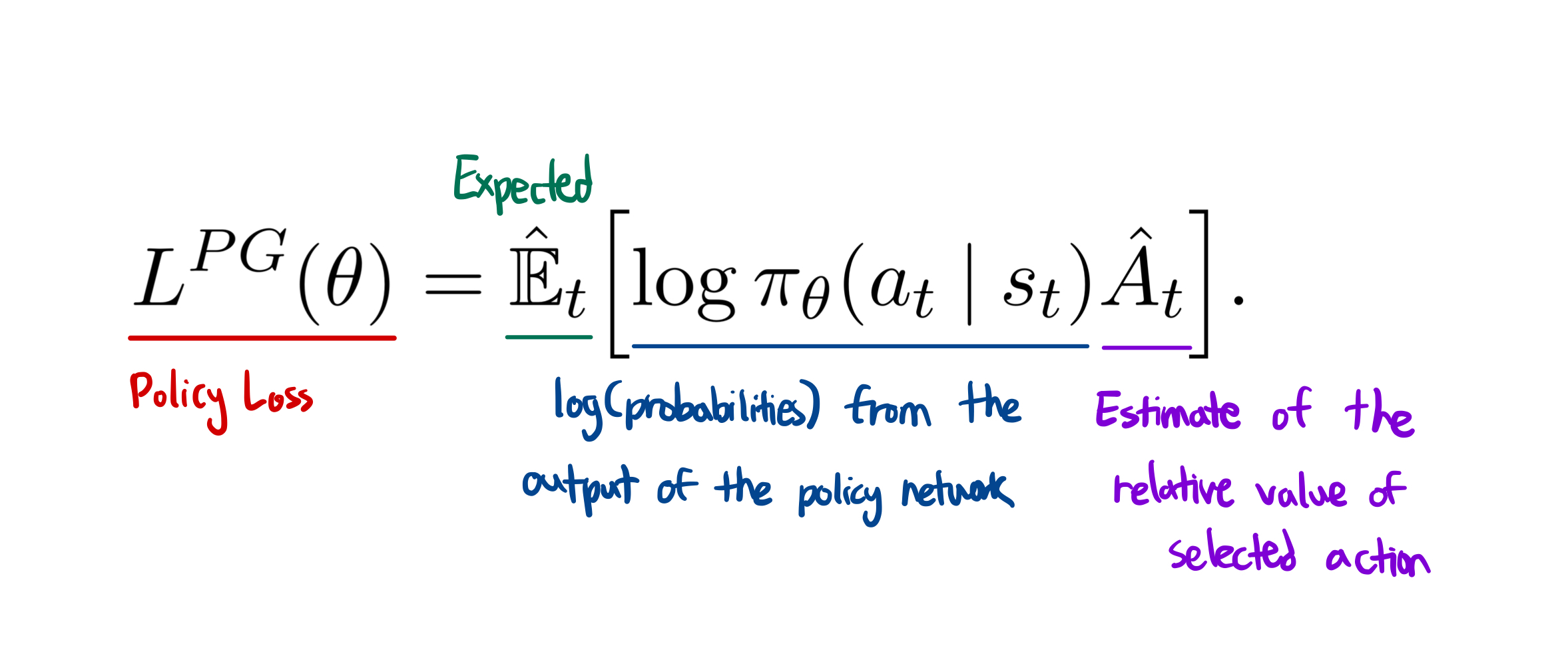
The policy is our neural network that takes the state observation from an environment as an input and suggest actions to take as an output. The advantage is an estimation, hence the hat over A, of the relative value for selected action in current state. It is computed as discounted reward(Q) - value function, where value function basically gives an estimate of discounted sum of reward. When training, this neural net representing the value function will frequently be updated using the experience our agent collects in an environment. However, that also means the value estimate will be very noisy due to the variance caused by the network; network is not always going to predict the exact value of that state.
Multiplying log probabilities of policy's output and advantage function gives us a clever optimization function. If advantage is positive, meaning the actions the agent took in the sample trajectory resulted in better than average return, policy gradient would be positive to increase the probability of selecting these actions again when we encounter a similar state. If advantage is negative, policy gradient would be negative to do the exact opposite.
As much appealing it is to constantly perform gradient descent steps in one batch of collected experience, it will often update the parameters so far outside of the range that leads to "destructively large policy updates."
Trust Region Policy Optimization
One of the approaches to prevent such destructive policy updates was Trust Region Policy Optimization (Schulman et al, 2015). In this paper, authors implemented an algorithm to limit the policy gradient step so it does not move too much away from the original policy, causing overly large updates that often ruin the policy altogether.
First, we define r(θ) as the probability ratio between the action under current policy and the action under the previous policy. 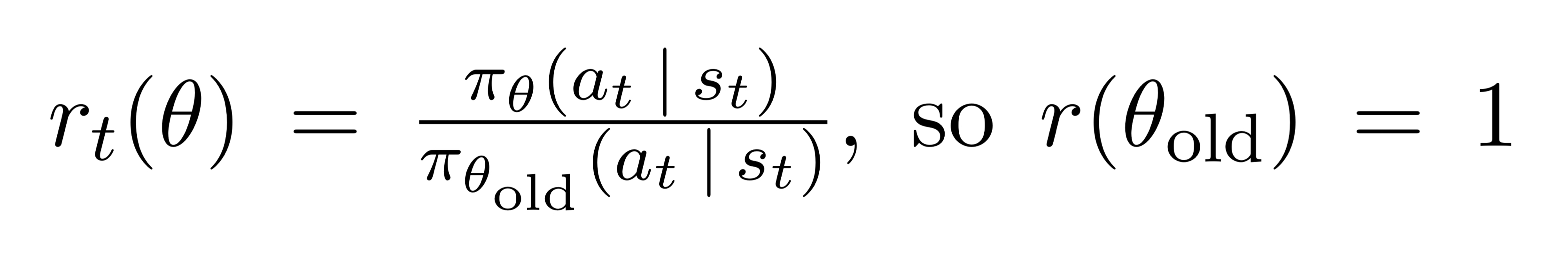
Given a sequence of sampled actions and states, r(θ) will be greater than one if the particular action is more probable for the current policy than it is for the old policy. It will be between 0 and 1 when the action is less probable for our current policy.
Now if we multiply this r(θ) with the previously mentioned advantage function, we get the TRPO's objective in a more readable format: 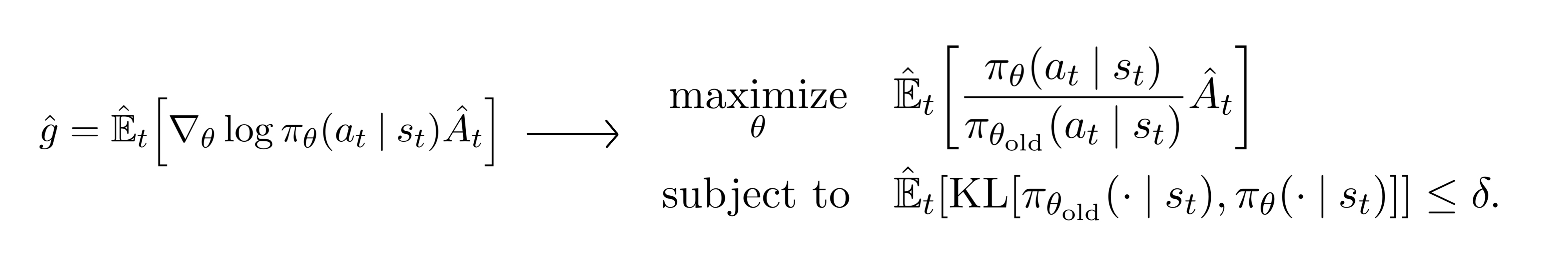
In this TRPO method, we notice that it is actually quite similar to the vanilla policy gradient method on the left. In fact, the only difference here is that the log operator is replaced with the probability of the action of current policy divided by the probability of the action under previous policy. Optimizing this objective function is identical otherwise.
Additionally, TRPO added a KL constraint limit the gradient step from moving the policy too far away from original policy. This results in the gradient staying in the region where we know everything works fine, hence the name 'trust region.' However, this KL constraint is known to add a overhead to our optimization process which sometimes lead to an undesirable training behavior.
PPO
Clipped Surrogate Objective
With the motives mentioned above, Proximal Policy Optimization attempts to simplify the optimization process while retaining the advantages of TRPO. One of this paper's main contribution is the clipped surrogate objective: 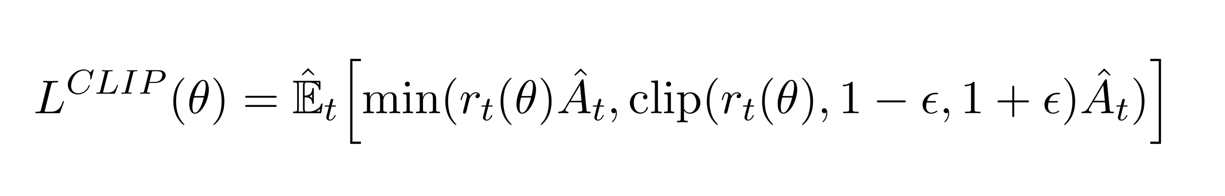
Here, we compute an expectation over the minimum of two terms: normal PG objective and clipped PG objective. The key component comes from the second term where a normal PG objective is truncated with a clipping operation between and , epsilon being the hyperparameter.
Because of the min operation, this objective behaves differently when advantage estimate is positive or negative.
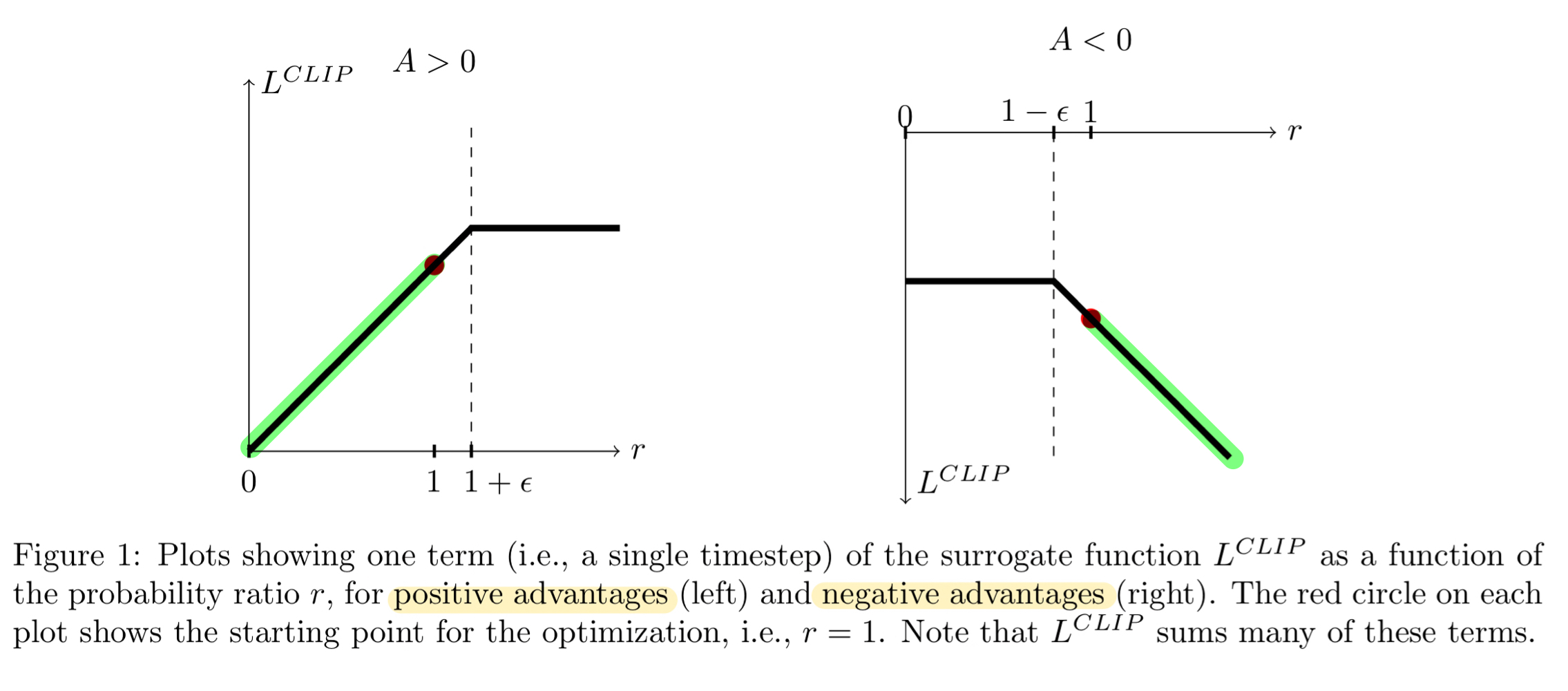
Let's first take a look at the left figure depecting postive advantage: the case when selected action had better-than-expected effect on the outcome. In the graph, the loss function flattens out when r gets too high or when action is a lot more likely under current policy than it was under old policy. We do not want to overdo the action update by taking a step too far, so we 'clip' the objective to prevent this as well as blocking the gradient with a flat line.
The same applies to the right figure when advantage estimate is negative. The loss function would flatten out when r goes near zero, meaning particular action is much less likely on current policy.
As clever this approach is, the clipping operation also helps us out for 'undoing' policy's mistakes. For example, the highlighted part in the right figure shows the region where last gradient step made the selected action a lot more probable while also making the policy worse as shown with a negative advantage. Thankfully, our clipping operation will kindly tell the gradient to walk the other direction in proportional to amount we messed up. This is the only part where the first term inside min() is lower than the second term, acting as a backup plan. And the most beautiful part is that PPO does all of this without having to compute additional KL constraints.
All of these ideas can be summarized in the final loss function by summing this clipped PPO objective and two additional terms:
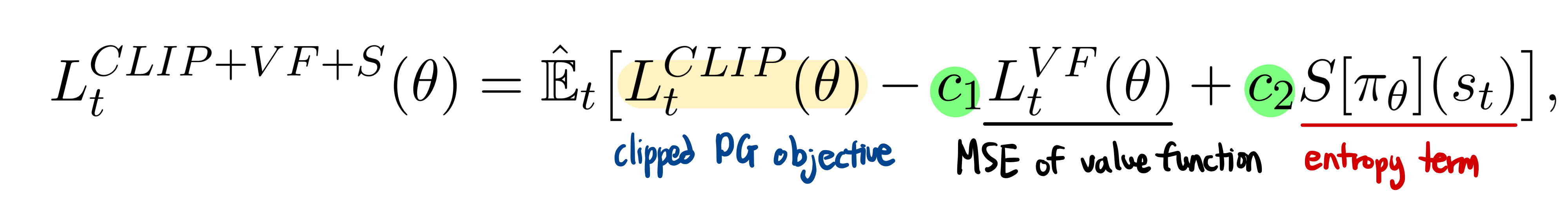
The c1 and c2 are hyperparameters. The first term is a mean square error of value function in charge of updating the baseline network. The second term, which may look unfamiliar, is an entropy term used to ensure enough exploration for our agents. This term will push the policy to behave more spontaneously until the other part of the objective starts dominating.
Multiple Epochs for Policy Updating
Finally, let's take a look at the algorithm altogether and its beauty of parallel actors:
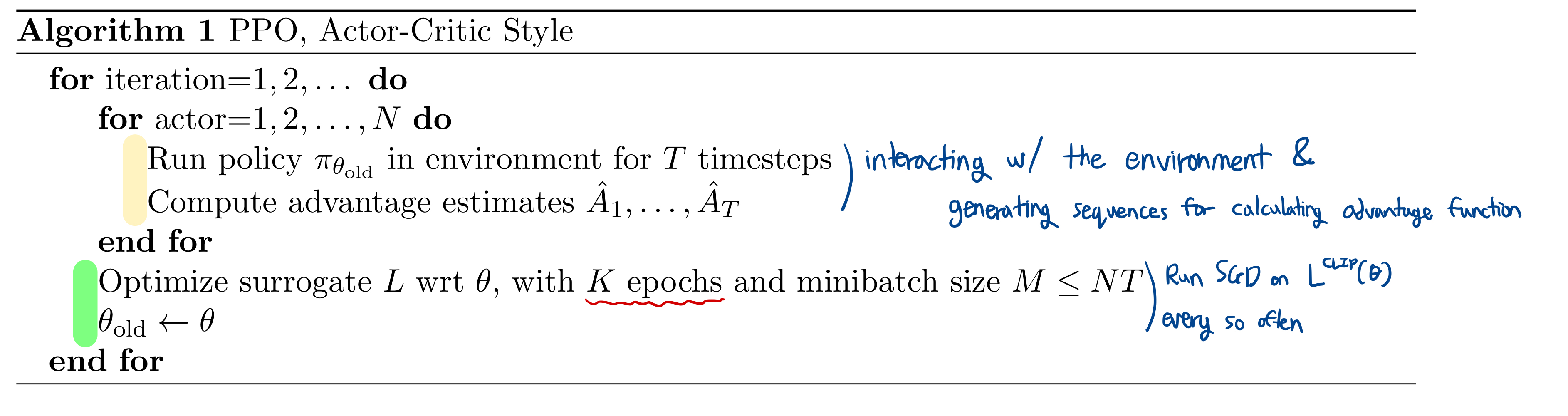
Algorithm consists of two large threads: the beige-thread and the green-thread. The beige-threads collect data, calculate advantage estimates, and sample mini-batches for the green-thread to use. One special take: these are done by N parallel actors each doing their own tasks independently.
Running multiple epochs of gradient descent on samples was uncommon because of the risk of destructively large policy updates. However, with the help of PPO's Clipped Surrogate Objective, we can take advantage of parallel actors to improve on sample efficiency.
Every once in a while, green-thread will fire and run Stochastic Gradient Descent on our clipped loss function. Another special take? We can run K epochs of optimization on the same trajectory sample. This was also hard to do pre-PPO due to the risk of taking large steps on local samples, but PPO prevents this while allowing us to learn more from each trajectory.